main topic interpreting results session command see also
You want to estimate the replacement rate of a certain valve on a fleet of 24 diesel engines.
1 Open the worksheet VSEAT.MTW.
2 Choose Stat > Reliability/Survival > Repairable System Analysis > Parametric Growth Curve.
3 In Variable/Start variables, enter Days.
4 In System ID, enter ID.
5 Click OK.
Session window output
Parametric Growth Curve: Days
System: ID
Model: Power-Law Process Estimation Method: Maximum Likelihood
Parameter Estimates
Standard 95% Normal CI Parameter Estimate Error Lower Upper Shape 4.00405 0.406 3.28239 4.88436 Scale 420.130 18.590 385.229 458.193
Test for Equal Shape Parameters Bartlett’s Modified Likelihood Ratio Chi-Square
Test Statistic 23.62 P-Value 0.425 DF 23
Trend Tests
MIL-Hdbk-189 Laplace’s TTT-based Pooled TTT-based Pooled Anderson-Darling Test Statistic 34.73 33.20 9.13 5.73 50.59 P-Value 0.000 0.000 0.000 0.000 0.000 DF 142 96 |
Graph window output
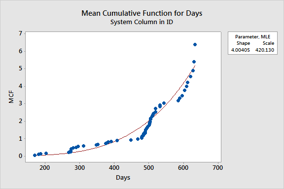
The estimate of the shape (4.004) is greater than 1, indicating that the failure rate is increasing. You can be 95% confident that the interval (3.282, 4.884) contains the true shape.
The test for equal shape parameters indicates that there is not enough evidence to say that the systems come from populations with different shapes (P-Value = 0.425). The pooled estimate of the shape is valid.
The tests for trend are all significant (P-Value = 0.000). This means that there is enough evidence to reject the null hypothesis that there is no trend in your data. You can conclude that the increasing trend is significant.
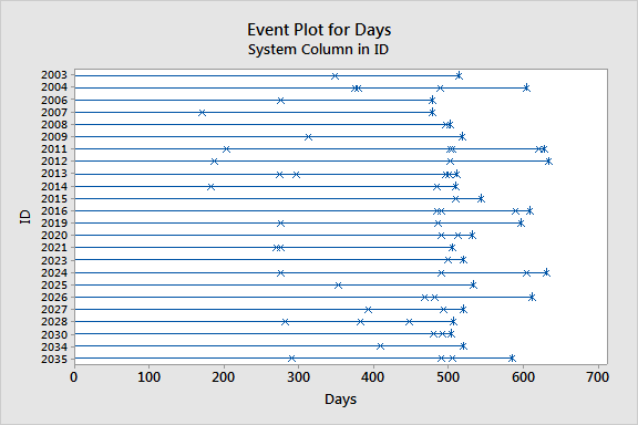
The event plot seems to show a pattern of failures that become more frequent as time goes on.
The plot of the MCF versus time shows a curve that is concave up. This plot is consistent with a shape that is greater than one, or a system that is deteriorating.