Inverse cumulative distribution function
Gives the value associated with a specific cumulative probability. Use
the inverse CDF to determine the value of the response associated with
a specific probability.
For example, an appliance manufacturer investigates failure times for
the heating element within its toasters. They want to determine the time
at which specific proportions of heating elements will fail so they can
set the warranty period. Heating element failure times follow a normal
distribution with a mean of 1000 hours and standard deviation of 300 hours.
The probability density function (PDF) describes the likelihood of each
possible failure time. The inverse CDF gives the corresponding failure
time for each cumulative probability under the PDF.
Use the inverse CDF to estimate the time by which 5% of the heating
elements will fail, the times between which 95% of all heating elements
will fail, or the time at which only 5% of the heating elements remain.
The inverse CDF for specific cumulative probabilities is equal to the
failure time at the right end of the shaded area under the PDF curve.
|

|
|

|
|

|
|
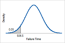
The time at which 5% of the heating elements are expected
to have failed is the inverse CDF of 0.05 or 506.5 hours. |
|
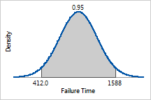
The times between which 95% of all heating elements are
expected to fail is the inverse CDF of 0.025 and the inverse CDF of 0.975
or 412 hours and 1588 hours. |
|
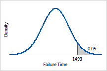
The time at which only 5% of the heating elements are
expected to remain is the inverse CDF of 0.95 or 1493 hours. |
