main topic interpreting results session command see also
Suppose you work for a company that manufactures engine windings for turbine assemblies. Engine windings may decompose at an unacceptable rate at high temperatures. You want to know - at given high temperatures - the time at which 1% of the engine windings fail. You plan to get this information by using Parametric Distribution Analysis (Right Censoring), which requires you to specify the distribution for your data. Distribution ID Plot - Right Censoring can help you choose that distribution.
First you collect failure times for the engine windings at two temperatures.
In the first sample, you test 50 windings at 80
1 Open the worksheet RELIABLE.MTW.
2 Choose Stat > Reliability/Survival > Distribution Analysis (Right Censoring) > Distribution ID Plot.
3 In Variables, enter Temp80 Temp100.
4 Choose Specify. Leave the default distributions as Weibull, lognormal, exponential, and normal.
5 Click Censor. Choose Use censoring columns and enter Cens80 Cens100 in the box. Click OK in each dialog box.
Session window output
Distribution ID Plot: Temp80, Temp100
Results for variable: Temp80
Goodness-of-Fit
Anderson-Darling Distribution (adj) Weibull 68.204 Lognormal 67.800 Exponential 70.871 Normal 68.305
Table of Percentiles
Standard 95% Normal CI Distribution Percent Percentile Error Lower Upper Weibull 1 10.0765 2.78453 5.86263 17.3193 Lognormal 1 19.3281 2.83750 14.4953 25.7722 Exponential 1 0.809731 0.133119 0.586684 1.11758 Normal 1 -0.549323 8.37183 -16.9578 15.8592
Weibull 5 20.3592 3.79130 14.1335 29.3273 Lognormal 5 26.9212 3.02621 21.5978 33.5566 Exponential 5 4.13258 0.679391 2.99422 5.70371 Normal 5 18.2289 6.40367 5.67790 30.7798
Weibull 10 27.7750 4.11994 20.7680 37.1463 Lognormal 10 32.1225 3.09409 26.5962 38.7970 Exponential 10 8.48864 1.39552 6.15037 11.7159 Normal 10 28.2394 5.48103 17.4968 38.9820
Weibull 50 62.6158 4.62515 54.1763 72.3700 Lognormal 50 59.8995 4.31085 52.0192 68.9735 Exponential 50 55.8452 9.18089 40.4622 77.0766 Normal 50 63.5518 4.06944 55.5759 71.5278
Table of MTTF
Standard 95% Normal CI Distribution Mean Error Lower Upper Weibull 64.9829 4.6102 56.5472 74.677 Lognormal 67.4153 5.5525 57.3656 79.225 Exponential 80.5676 13.2452 58.3746 111.198 Normal 63.5518 4.0694 55.5759 71.528
Results for variable: Temp100
Goodness-of-Fit
Anderson-Darling Distribution (adj) Weibull 17.339 Lognormal 17.253 Exponential 18.879 Normal 17.781
Table of Percentiles
Standard 95% Normal CI Distribution Percent Percentile Error Lower Upper Weibull 1 2.98186 1.26067 1.30201 6.82903 Lognormal 1 6.87764 1.61698 4.33827 10.9034 Exponential 1 0.502517 0.0861809 0.359063 0.703284 Normal 1 -18.8392 8.80960 -36.1057 -1.57266
Weibull 5 8.17115 2.36772 4.63056 14.4189 Lognormal 5 11.3181 2.07658 7.89954 16.2162 Exponential 5 2.56466 0.439836 1.83253 3.58931 Normal 5 -0.298373 6.86755 -13.7585 13.1618
Weibull 10 12.7534 2.97772 8.07016 20.1543 Lognormal 10 14.7606 2.35025 10.8036 20.1667 Exponential 10 5.26803 0.903459 3.76416 7.37272 Normal 10 9.58565 5.95326 -2.08252 21.2538
Weibull 50 40.8900 4.73799 32.5827 51.3153 Lognormal 50 37.6636 4.43620 29.8995 47.4439 Exponential 50 34.6574 5.94369 24.7637 48.5038 Normal 50 44.4516 4.37371 35.8793 53.0240
Table of MTTF
Standard 95% Normal CI Distribution Mean Error Lower Upper Weibull 45.9448 4.87525 37.3177 56.5663 Lognormal 49.1969 6.91761 37.3465 64.8076 Exponential 50.0000 8.57493 35.7265 69.9761 Normal 44.4516 4.37371 35.8793 53.0240
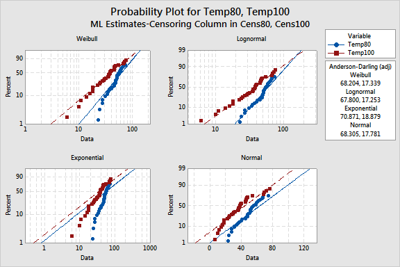
Distribution ID Plot for Temp80, Temp100 |
Graph window output

The points fall approximately on the straight line on the lognormal probability plot, so the lognormal distribution would be a good choice when running the parametric distribution analysis. You can also compare the Anderson-Darling goodness-of-fit values to determine which distribution best fits the data. A smaller Anderson-Darling statistic means that the distribution provides a better fit. Here, the Anderson-Darling values for the lognormal distribution are lower than the Anderson-Darling values for other distributions, thus supporting your conclusion that the lognormal distribution provides the best fit.
The table of percentiles and MTTFs allow you to see how your conclusions may change with different distributions.
| Minitab help | Stat | Graph | SixSigma | DOE | Glossary | Reliability | SPC,MSA,CPK | ||
|
|||||||||